
Transmission and Absorption of X-rays in matter#
The purpose of this guide is to present an overview of the roentgen.absorption module which provides for the calculation of the transmission and absorption of X-rays through and by various materials.
Mass Attenuation Coefficient#
The primary component that mediates the x-ray attenuation through a material is its mass attenuation coefficient.
These tabulated values can be inspected using the roentgen.absorption.MassAttenuationCoefficient object.
To create one:
from roentgen.absorption import MassAttenuationCoefficient
si_matten = MassAttenuationCoefficient('Si')
Tabulated values for all elements are provided as well as additional specialized materials. These data are provided by the U.S National Institute of Standards and Technology (NIST) and range from 1 keV to 20 MeV. Elements can be specificied by their symbol name or by their full name (e.g. Si, Silicon). A list of all of the elements is provided by:
roentgen.elements
Specialized materials, referred to as compounds, are also available. A complete list is provided by:
roentgen.compounds
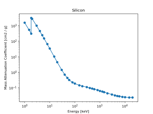
Here is the mass attenuation coefficient data for Silicon.
import astropy.units as u
import matplotlib.pyplot as plt
from roentgen.absorption import MassAttenuationCoefficient

si_matten = MassAttenuationCoefficient('Si')
plt.plot(si_matten.energy, si_matten.data, 'o-')
plt.yscale('log')
plt.xscale('log')
plt.xlabel('Energy [' + str(si_matten.energy[0].unit) + ']')
plt.ylabel('Mass Attenuation Coefficient [' + str(si_matten.data[0].unit) + ']')
plt.title(si_matten.name)
plt.show()
(Source code, png, hires.png, pdf)
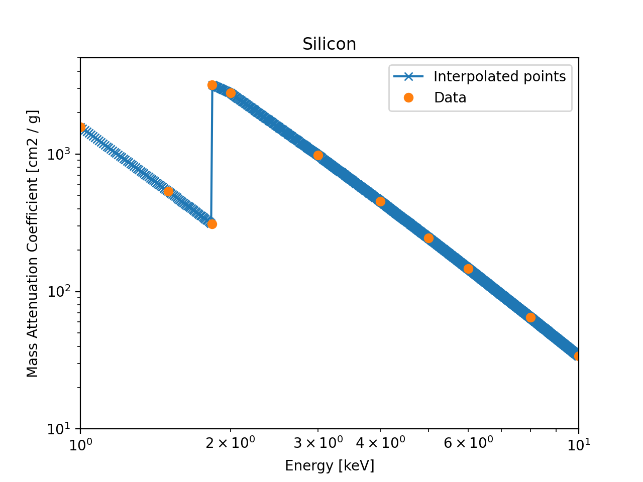
You can get the interpolated value at any other point
import astropy.units as u
import matplotlib.pyplot as plt
from roentgen.absorption import MassAttenuationCoefficient

si_matten = MassAttenuationCoefficient('Si')

energy = u.Quantity(np.arange(1, 10, 0.01), 'keV')
interpol_atten = si_matten.func(energy)

plt.plot(energy, interpol_atten, 'x-', label='Interpolated points')
plt.plot(si_matten.energy, si_matten.data, 'o', label='Data')

plt.xlim(1, 10)
plt.ylim(10, 5000)
plt.yscale('log')
plt.xscale('log')
plt.xlabel(f'Energy [{si_matten.energy[0].unit}]')
plt.ylabel(f'Mass Attenuation Coefficient [{si_matten.data[0].unit}]')
plt.title(si_matten.name)
plt.legend()
plt.show()
(Source code, png, hires.png, pdf)
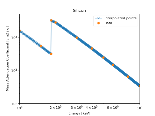
Be careful that you interpolate with sufficient resolution to make out complex edges if high accuracy is required.
Material#
In order to determine the x-ray attenuation through a material the roentgen.absorption.Material object is provided.
This object can be created by providing the thickness of the material through which the x-rays are interacting.
The thickness must be given by a Quantity.
For example, a 500 micron thick layer of Aluminum can be created like so:
al = Material('Al', 500 * u.micron)
An optional density can also be provided.
A default density is assumed if none is provided.
Default values can be found in elements.csv for elements or in compounds_mixtures.csv for compounds.
Warning
Elements beyond z = 92 are not supported by this module.
To inspect the density:
al.density
Using this object it is possible to get the absorption and transmission as a function of energy:
energy = u.Quantity(np.arange(1,30), 'keV')
al.transmission(energy)
al.absoprtion(energy)
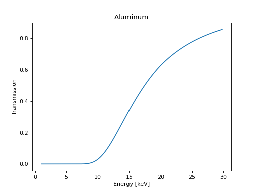
Here is a plot of the transmission of x-rays through 500 micron of Aluminum, a standard thickness for electronics boxes. The transmission and absorption is given on a scale from 0 (no absorption or no transmission) to 1 (complete absorption or complete transmission).
import numpy as np
import matplotlib.pyplot as plt
import astropy.units as u

from roentgen.absorption import Material

al = Material('Al', 500 * u.micron)
energy = u.Quantity(np.arange(1, 30, 0.2), 'keV')

plt.plot(energy, al.transmission(energy))
plt.ylabel('Transmission')
plt.xlabel('Energy [' + str(energy.unit) + ']')
plt.title(al.name)
plt.show()
(Source code, png, hires.png, pdf)

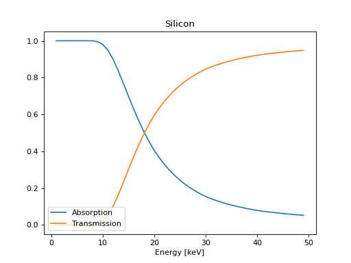
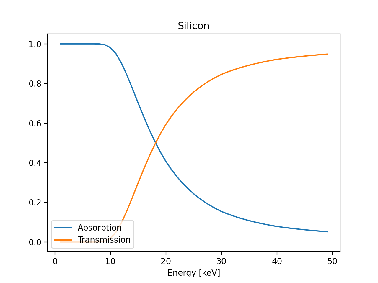
From the above plot, one can see that the this thickness of Aluminum blocks almost all x-rays below about 7 keV. The relationship between transmission and absorption can be seen in the following plot for 500 microns of Silicon, a standard thickness for a soft x-ray detector.
import numpy as np
import matplotlib.pyplot as plt
import astropy.units as u

from roentgen.absorption import Material

si = Material('Si', 500 * u.micron)
energy = u.Quantity(np.arange(1, 50), 'keV')

plt.plot(energy, si.absorption(energy), label='Absorption')
plt.plot(energy, si.transmission(energy), label='Transmission')
plt.xlabel('Energy [' + str(energy.unit) + ']')
plt.title(si.name)
plt.legend(loc='lower left')
plt.show()
(Source code, png, hires.png, pdf)

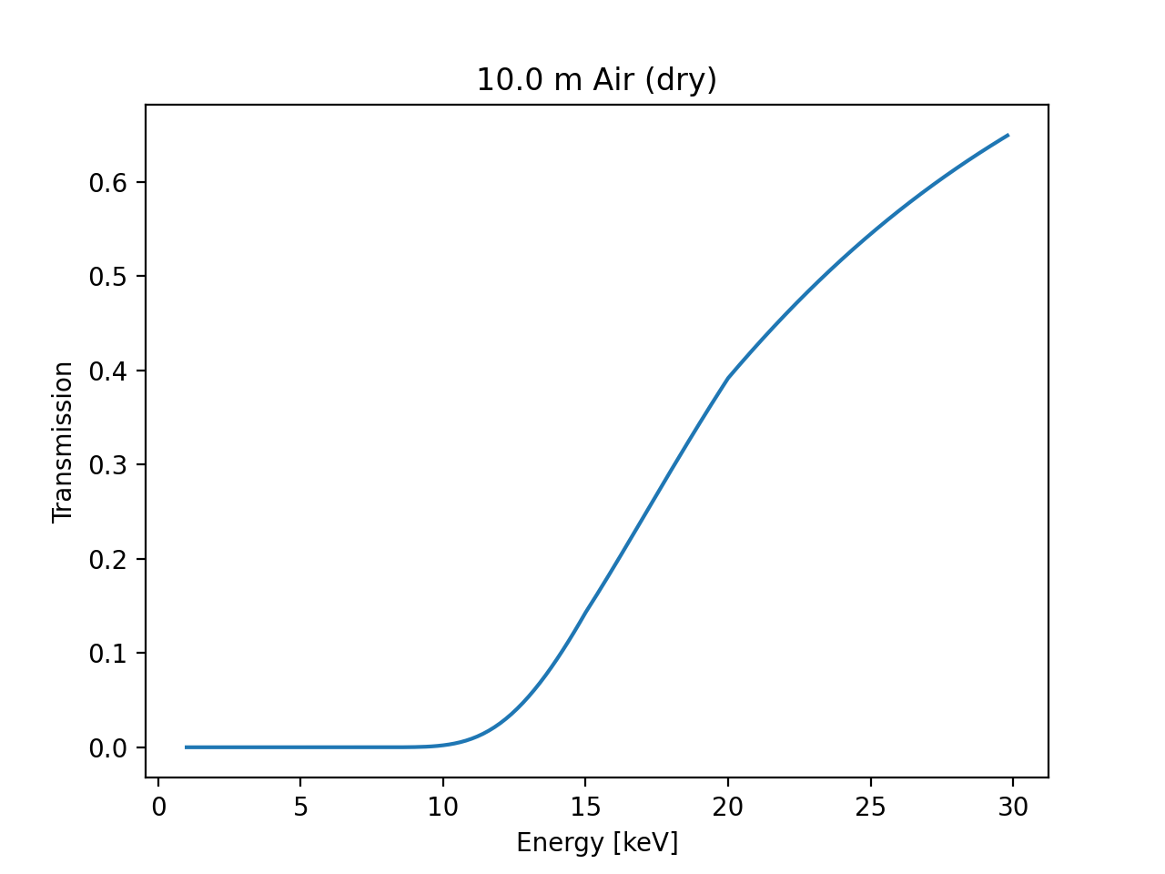
Besides elements, a number of compounds and mixtures are also available. As a simple example, here is the transmission of x-rays through 10 meters of air.
import numpy as np
import matplotlib.pyplot as plt
import astropy.units as u

from roentgen.absorption import Material

thickness = 10 * u.m
air = Material('air', thickness)
energy = u.Quantity(np.arange(1, 30, 0.2), 'keV')

plt.plot(energy, air.transmission(energy))
plt.ylabel('Transmission')
plt.xlabel('Energy [' + str(energy.unit) + ']')
plt.title(f"{thickness} {air.name}")
plt.show()
(Source code, png, hires.png, pdf)
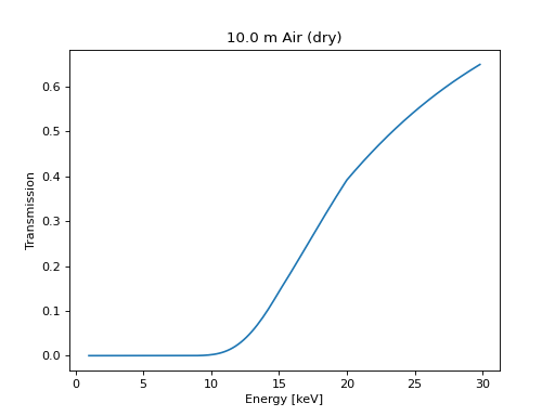
This plot shows that air, though not a dense material, does block low energy x-rays over long distances.
For convenience, the function density_ideal_gas is provided which can calculate the density of a gas given a pressure and temperature.
It is also possible to create custom materials using a combination of elements and compounds:
>>> import astropy.units as u
>>> from roentgen.absorption import Material
>>> steel = Material({"Fe": 0.98, "C": 0.02}, 1 * u.cm)
>>> bronze = Material({"Cu": 0.88, "Sn": 0.12}, 1 * u.cm)
>>> salt_water = Material({"water": 0.97, "Na": 0.015, "Cl": 0.015}, 1 * u.cm)
The fractions need not be normalized. It will normalize them for you. The density will be calculated automatically using the known densities but this is likely not a good assumption so you should provide your own density:
>>> bronze = Material({"Cu": 0.88, "Sn": 0.12}, 1 * u.cm)
>>> bronze.density
<Quantity 8762. kg / m3>
>>> bronze = Material({"Cu": 0.88, "Sn": 0.12}, 1 * u.cm, density=8.73 * u.g / u.cm**-3)
Stack#
Materials can be added together to form more complex optical paths.
If two or more materials are added together they form a roentgen.absorption.Stack.
A simple example is the transmission through air and then through a thermal blanket composed of a thin layer of mylar and Aluminum:
optical_path = Material('air', 2 * u.m) + Material('mylar', 5 * u.micron) + Material('Al', 5 * u.micron)
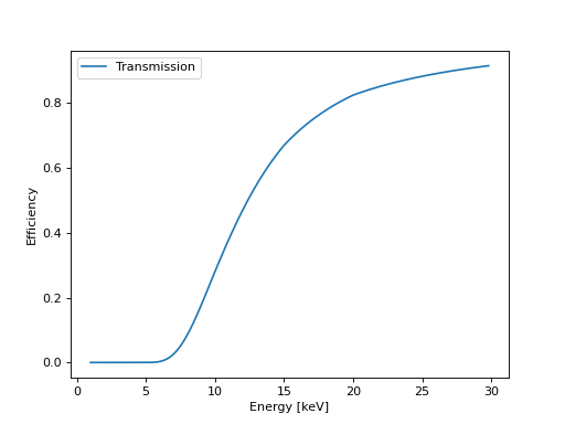
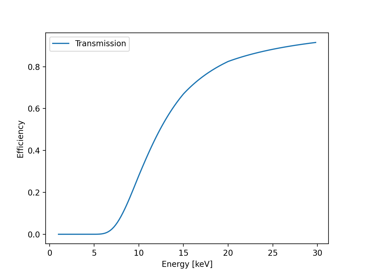
This new object also provides transmission and absorption of the combination of these materials. Here is a plot of that transmission over energy
import numpy as np
import matplotlib.pyplot as plt
import astropy.units as u

from roentgen.absorption import Material

optical_path = Material('air', 2 * u.m) + Material('mylar', 5 * u.micron) + Material('Al', 5 * u.micron)
energy = u.Quantity(np.arange(1, 30, 0.2), 'keV')

plt.plot(energy, optical_path.transmission(energy), label='Transmission')
plt.ylabel('Efficiency')
plt.xlabel(f'Energy [{energy.unit}]')
plt.legend(loc='upper left')
plt.show()
(Source code, png, hires.png, pdf)

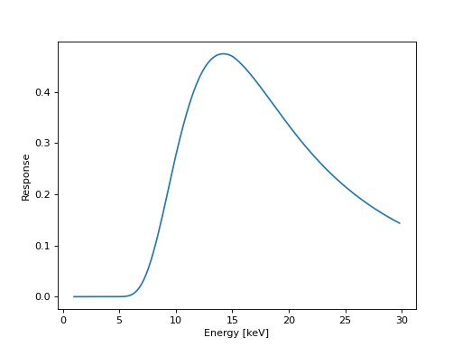
Frequently, it is useful to consider the response function of a particular detector which includes absorption through materials in front of a detector. This can be calculated by multiplying the transmission of the materials before the detector with the absorption of the detector material.
To simplify this process, the roentgen.absorption.Response class is provided.
The following example uses the same optical path as defined above and assumes a Silicon detector.
import numpy as np
import astropy.units as u
import matplotlib.pyplot as plt
from roentgen.absorption import Material, Response, Stack

optical_path = Stack([Material('air', 2 * u.m), Material('mylar', 5 * u.micron), Material('Al', 5 * u.micron)])
detector = Material('Si', 500 * u.micron)
resp = Response(optical_path=optical_path, detector=detector)
energy = u.Quantity(np.arange(1, 30, 0.2), 'keV')

plt.plot(energy, resp.response(energy))
plt.xlabel(f'Energy [{energy.unit}]')
plt.ylabel('Response')
plt.show()
(Source code, png, hires.png, pdf)

This plot shows that the peak efficiency for this detector system is less than 50% and lies around 15 keV.